Logistics Regression is a simple and powerful model for machine learning classification algorithms. As simple as it is, logistics regression for classification could be tricky, and to find an acceptable model, someone might have to go run several iterations.
On the web sphere, we see various publications and tutorials showing 99% accuracy or 90% f1 score. While those results might be achievable readers must be extremely careful about the context, the data used, the application, etc... Without applying some professional techniques, the best accuracy is 72% and the highest optimized f1 score is 52%.
Note: Though tempting, Logistic Regression could NOT explain causality, it is mostly used as a predictive function.
There are 3 important points with Logistic Regression:
- Confusion Matrix (False Positive could be very dangerous)
- Class Imbalance
- Model Performance criteria or scoring
Logistic Regression is a linear model derived to solve classification problems. Logistic regression falls under supervised machine learning type modeling. This means we train a historical dataset to predict results. By definition, unsupervised do not need training.
What kind of problems does Logistics Regression Solve?
1 - Binary Logistics Regression
The target value has only two categories for example:
- (Yes / No)
- (1 / 0)
- (True / False)
- (Spam / Safe)
Some real-life applications would be Healthcare: Predict if a patient has a disease i.e. machine learning to predict diabetes is very famous. These types of binary output algorithms have been used by financial institutions to predict if a person would default on their loan payment, or if a credit card transaction is fraudulent. E-commerce uses the likelihood score above 70% to recommend upselling and cross-selling products, this has been a fantastic marketing tactic to boost sales.
2 - Multinomial Logistics Regression
The target has more than two categories that are not in a specific order for example:
- (Banana / Apple / Peach)
- (Lion / Panda / Bear)
A real-life application would be the famous IRIS classification. Recently the farming industry is upgrading many businesses with machine learning classifiers.
3 - Ordinal Logistics Regression
The target value has more than 2 categories with intrinsic grading values:
- (Excellent / Very Good / Good)
- (5 Stars / 4 Stars / 3 Stars)
A real-Life application would be a business review and rating
Model Evaluation for Logistic Regression
Although Logistic Regression is easy to use and fast at making predictions model evaluation is counterintuitive
1 - Accuracy
It is the most commonly used method to evaluate how well the model is predicting results. Many data scientists compare Accuracy to the Null Accuracy to rank model performance. In practice when looking at the confusion matrix, someone could quickly conclude that accuracy is not the preferred performance evaluation method.
2 - Classification Report
The classification report is the better method for comparing the performance of Logistics Regression models. Two models might have equal Accuracy but one model with higher precision and recall values is a far superior model.
The Dataset
There are many datasets to choose from. To keep it simple we selected the dataset provided by UCLA which could be downloaded from here. The dataset is simple and common, it shows the decision of admission versus not based on GRE and GPA. The rank is a college classification metric with rank 1 being the best down to 4. It is worth testing if the college ranking metric is influencing the output and in particular if we reverse the ranking from 4 to 1 where 1 would be the best college.
Problem Statement
Could we use logistic regression to predict the admission of a student based on GRE, GPA, and college rank?
Data Preparation for Logistic Regression
- Set and inspect the data (missing values, duplicates, outliers, features...)
- Define the features (independent variables)
- Decide if dummy variables are needed
- Set the dependent variable
- Raw data or scaled or standardized data?
- Split the data (80/20, 75/25, 70/30) for this example they all work
- Plot the data pairwise
- Check for colinearity
- Check for imbalance in the dependent variables (is the number of zero equal to the number of one)?
- Fine Tune the algorithm if necessary
Here is the Logistic Regression Python Code Complete, with all the comments it should be self-explanatory. And for the sake of clarity let's call the first run Benchmarking
Benchmarking Admission Logistics Regression
import pandas as pd
from sklearn.model_selection import train_test_split
from sklearn.linear_model import LogisticRegression

#import data
df = pd.read_csv("admission.csv")

X = df.iloc[:,df.columns != 'admit']
y = df['admit']

#Split data into test and train
X_train,X_test,y_train,y_test = train_test_split(X,y,test_size=0.25,random_state=0)

logistic_regression= LogisticRegression()
logistic_regression.fit(X_train,y_train)

y_pred=logistic_regression.predict(X_test)

from sklearn.metrics import  confusion_matrix, accuracy_score, classification_report
from matplotlib import pyplot as plt
import seaborn as sns

cfm=confusion_matrix(y_test,y_pred)
plt.title("Confusion Matrix")
sns.heatmap(cfm, annot=True, fmt='',cbar=False)
plt.show()

TP = cfm[1,1]
TN = cfm[0,0]
FP = cfm[1,0]
FN = cfm[0,1]

print ('True Positive: ', TP)
print ('True Negative: ', TN)
print ('False Positive: ', FP)
print ('False Negative: ', FN)

print('Confusion Matrix:  \n', cfm)
print('Accuracy: ', accuracy_score(y_test, y_pred)*100,'%')
print ('Manual Accuracy: ', ((TP+TN)/(TP+TN+FP+FN))*100,'%')
print('Class Report: \n', classification_report(y_test, y_pred))
Before we explain the result of the confusion matrix it is critical to say that there are different index conventions for the confusion matrix. The placement of the axis of the confusion matrix of Wikipedia is different from the scikit learn confusion matrix library we used here.
The result of the confusion matrix is:
- True Positive TP = 8
- True Negative TN = 64
- False Positive FP = 27
- False Negative FN = 4
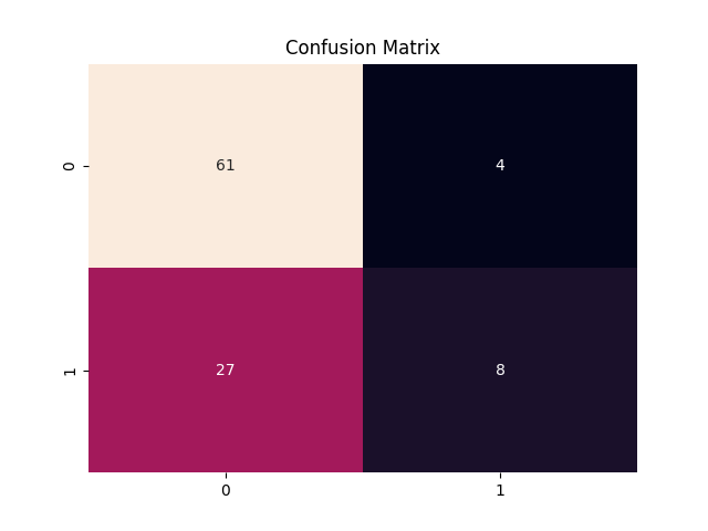
Logistic regression is a classification algorithm in this case the output class is binary either admit (1) or not admit (0). From the confusion matrix, the predicted admission versus the actual admission is calculated and then plotted. The confusion matrix provides a 2x2 matrix where index (1,1) is True Positive, (0,0) is True Negative, (1,0) is False Positive and (0,1) is False Negative. The accuracy of the model is simply calculated by the (TP+TN)/(TP+TN+FP+FN).
Extreme care must be taken when using Logistics Regression, for critical applications such as healthcare, the military, forensic work, etc... an impressive 98% accurate model could lead to the death of people we have seen cases where the confusion matrix False Positive and False Negative constitute a big chunk. A 1% of 10,000 people is about 100 people with the wrong prediction that is way too much.
Our benchmark model score is 69% which might be good for noncritical models such as junk mail filtering.
True Positive:  8
True Negative:  61
False Positive:  27
False Negative:  4
Confusion Matrix:
 [[61  4]
 [27  8]]
Accuracy:  69.0 %
Manual Accuracy:  69.0 %
Class Report:
               precision    recall  f1-score   support

           0       0.69      0.94      0.80        65
           1       0.67      0.23      0.34        35

    accuracy                           0.69       100
   macro avg       0.68      0.58      0.57       100
weighted avg       0.68      0.69      0.64       100
Class Imbalance
Care must be taken when implementing Logistic Regression, in some datasets with binary 0,1 responses, the output could be biased such that 98% of the target is either 0 or 1. In which case the score of the model is 98% which in theory is a perfect performance. In that case, the model is good but the physical problem is not properly defined and the dataset is known to have a high Class Imbalance.
In our admission dataset, the admission rate is 32% with label '1' and the rejection rate is 68% with label '0'. When building the model, the computation might induce a bias toward the majority class and the model might erroneously predict more '0' than expected.
How to handle Class Imbalance in Logistics Regression?
The first step is to recognize that there is a Class Imbalance, and for 68% vs 32% distribution there is a Class Imbalance. There are several approaches to account for Imbalance in a dataset. Proportionally, we could reduce the frequency of the majority class, or vice versa we might increase the frequency of the minority class. In this preprocessing step the aim is to obtain the same number of observations of both classes for model development purposes. The proportionality could be implemented using a weighting factor.
Depending on the software package being used, some logistic regression software supports the weighing factor natively. In our case the weighing class is built-in and we will use it for potentially better performance.
In our improved model, we will also use some Tuning Parameters known as hyperparameter tuning. While it seems a little cumbersome having to go back and forth this method has a lot of potentials.
In this section, we will run the code with a manual class weight that represents the inverse ratio of Class 1 and Class 0 i.e. 0.68 vs 0.32.
import pandas as pd
import numpy as np
from sklearn.model_selection import train_test_split
from sklearn.linear_model import LogisticRegression
from sklearn.metrics import  confusion_matrix, accuracy_score, classification_report

#import data
df = pd.read_csv("admission.csv")

X = df.iloc[:,df.columns != 'admit']
y = df['admit']

#Split data into test and train
X_train,X_test,y_train,y_test = train_test_split(X,y,test_size=0.25,random_state=42)

#Benchmarking starting the weight class with reversed proportions
LR_Model_Base =LogisticRegression(class_weight={0:0.32,1:0.68})
LR_Model_Base.fit(X_train,y_train)
y_pred=LR_Model_Base.predict(X_test)
cfm=confusion_matrix(y_test,y_pred)
print('Confusion Matrix:  \n', cfm)
print('Accuracy: ', accuracy_score(y_test, y_pred)*100,'%')
print('Class Report: \n', classification_report(y_test, y_pred))
Expecting the accuracy result to go up? Actually at 60% accuracy went down by 9% percentage points with respect to the first trial.
The only thing we changed with respect to the first run is class weight to account for the Class Imbalance in the data set
Confusion Matrix:
 [[39 27]
 [13 21]]
Accuracy:  60.0 %
Class Report:
               precision    recall  f1-score   support

           0       0.75      0.59      0.66        66
           1       0.44      0.62      0.51        34

    accuracy                           0.60       100
   macro avg       0.59      0.60      0.59       100
weighted avg       0.64      0.60      0.61       100
Is there a better way to estimate the class weight?
Is there a way to increment through class weight sets and find an optimal point?
Using Grid Search cross-validation the system will run through many parameter sets to suggest better argument sets for Logistics Regression.
import pandas as pd
import numpy as np
from sklearn.model_selection import train_test_split
from sklearn.linear_model import LogisticRegression
from sklearn.metrics import  confusion_matrix, accuracy_score, classification_report

#import data
df = pd.read_csv("admission.csv")

X = df.iloc[:,df.columns != 'admit']
y = df['admit']

#Split data into test and train
X_train,X_test,y_train,y_test = train_test_split(X,y,test_size=0.25,random_state=42)

LR_Model= LogisticRegression()
#0.99 converges better than 1, no more 100 for faster code
CIW = np.linspace(0.0,0.99,100)

param = dict()
param['solver'] = ['liblinear', 'saga', 'sag','lbfgs', 'newton-cg']
param['penalty'] = ['l1', 'l2', 'elasticnet','none']
param['C'] = [1e-5, 1e-4, 1e-3, 1e-2, 1e-1, 1, 10, 100]
param['class_weight'] = [{0:x,1:1.0-x} for x in CIW]

from sklearn.model_selection import StratifiedKFold
from sklearn.model_selection import GridSearchCV
# Cross Validation 5 folds
folds = StratifiedKFold(n_splits=5, shuffle=True, random_state=42)

#Gridsearch for hyperparam tuning
GS= GridSearchCV(LR_Model, param, n_jobs=-1, scoring='accuracy', cv=folds, return_train_score=True)
GS.fit(X_train,y_train)
print("Achievable score: ", GS.best_score_)
print("Estimator: ", GS.best_estimator_)
print("Hyperparameters: ", GS.best_params_)
Note Setting the Grid Search with many parameters as we did in the above example will take some time to converge, any time from a few minutes up to some hours - so be patient and methodically try to reduce the input parameters that are not needed.
As shown the output will provide the optimized Logistic Regression argument.
Achievable score:  0.7166666666666667
Estimator:  LogisticRegression(C=10, class_weight={0: 0.53, 1: 0.47})
Hyperparameters:  {'C': 10, 'class_weight': {0: 0.53, 1: 0.47}, 'penalty': 'l2'}
From the hyperparameters we got from the previous trial, we could now edit the argument and see if we get a better performance and accuracy result.
import pandas as pd
import numpy as np
from sklearn.model_selection import train_test_split
from sklearn.linear_model import LogisticRegression
from sklearn.metrics import  confusion_matrix, accuracy_score, classification_report

#import data
df = pd.read_csv("admission.csv")

X = df.iloc[:,df.columns != 'admit']
y = df['admit']

#Split data into test and train
X_train,X_test,y_train,y_test = train_test_split(X,y,test_size=0.25,random_state=42)

# With Hypertuning Paramaters
LR_Model= LogisticRegression(C=10,class_weight={0:0.53,1:0.47},penalty="l2")
LR_Model.fit(X_train,y_train)

y_pred=LR_Model.predict(X_test)

cfm=confusion_matrix(y_test,y_pred)

print('Confusion Matrix:  \n', cfm)
print('Accuracy: ', accuracy_score(y_test, y_pred)*100,'%')
print('Class Report: \n', classification_report(y_test, y_pred))
I warned unless done right tuning might take forever.
With 70% accuracy, the model now is better than the 60% we have prior and the best we have achieved so far in this article.
Another observation is that in the Confusion Matrix the numbers of true positive and false positive and true positive have changed dramatically.
Confusion Matrix:
 [[65  1]
 [29  5]]
Accuracy:  70.0 %
Class Report:
               precision    recall  f1-score   support

           0       0.69      0.98      0.81        66
           1       0.83      0.15      0.25        34

    accuracy                           0.70       100
   macro avg       0.76      0.57      0.53       100
weighted avg       0.74      0.70      0.62       100
We changed the hypertuning a bit to optimize for precision and recall as shown.
import pandas as pd
import numpy as np
from sklearn.model_selection import train_test_split
from sklearn.linear_model import LogisticRegression
from sklearn.metrics import  confusion_matrix, accuracy_score, classification_report

#import data
df = pd.read_csv("admission.csv")

X = df.iloc[:,df.columns != 'admit']
y = df['admit']

#Split data into test and train
X_train,X_test,y_train,y_test = train_test_split(X,y,test_size=0.25,random_state=42)

LR_Model= LogisticRegression()
#0.99 converges better than 1, no more 100 for faster code
CIW = np.linspace(0.0,0.99,100)

param = dict()
param['solver'] = ['liblinear', 'saga', 'sag','lbfgs', 'newton-cg']
param['penalty'] = ['l1', 'l2', 'elasticnet','none']
param['C'] = [1e-5, 1e-4, 1e-3, 1e-2, 1e-1, 1, 10, 100]
param['class_weight'] = [{0:x,1:1.0-x} for x in CIW]

from sklearn.model_selection import StratifiedKFold
from sklearn.model_selection import GridSearchCV
# Cross Validation 5 folds
folds = StratifiedKFold(n_splits=5, shuffle=True, random_state=42)

#Gridsearch for hyperparam tuning
GS= GridSearchCV(LR_Model, param, n_jobs=-1, scoring='f1', cv=folds, return_train_score=True)
GS.fit(X_train,y_train)
print("Achievable score: ", GS.best_score_)
print("Estimator: ", GS.best_estimator_)
print("Hyperparameters: ", GS.best_params_)
And the result would be
Confusion Matrix:
 [[28 38]
 [ 8 26]]
Accuracy:  54.0 %
Class Report:
               precision    recall  f1-score   support

           0       0.78      0.42      0.55        66
           1       0.41      0.76      0.53        34

    accuracy                           0.54       100
   macro avg       0.59      0.59      0.54       100
weighted avg       0.65      0.54      0.54       100
Now with this result, some can notice a significant increase in f1 score namely the precision and recall for class "1" category admitted. The precision and recall are much better than the benchmark run. It looks that no matter what we do the model is not good enough with 54% accuracy.