Linear Regression, a cornerstone of data analysis, boasts a rich history dating back over a century. Introduced by luminaries like Francis Galton and Karl Pearson, its roots trace back to 1875 and 1920, laying the groundwork for concepts like Pearson Correlation.
While purists statisticians may debate its categorization within the realms of statistics rather than Machine Learning, let's not allow ourselves to become entangled in mere semantics. The true essence lies in its transformative potential, transcending disciplinary boundaries to become an integral part of the Machine Learning landscape.
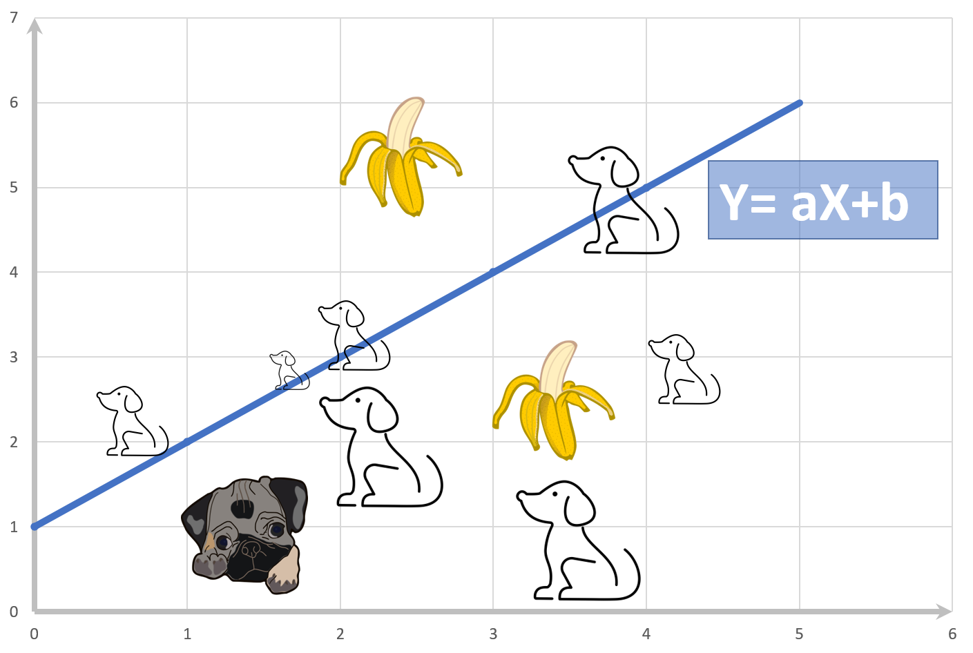
Linear Regression: A Pillar of Machine Learning
But Linear Regression for puppies and bananas? Indeed, Linear Regression occupies a pivotal position within the realm of Machine Learning, offering predictive capabilities at its very core. Unlike traditional statistical approaches, Machine Learning algorithms adopt a forward-thinking strategy, leveraging data partitioning techniques by split the data into a training data subset, and a test subset to assess model performance proactively.
And the beauty of it all? Implementing Linear Regression is a breeze, whether it's a few lines of Python code or a series of keystrokes in Excel. Its accessibility underscores its relevance in the ever-evolving world of Machine Learning.
Delving Deeper: Unraveling the Science Behind Linear Regression
In this discourse, our focus transcends the mere execution of algorithms. Instead, we embark on a journey to unravel the intricate interplay of physical meaning, scientific underpinnings, and mathematical elegance. It's about more than just crunching numbers; it's about solving real-world problems with precision and finesse.
So, as we navigate through the complexities of Linear Regression, let's not merely scratch the surface. Instead, let's delve deeper, uncovering the profound insights and transformative potential that lie at the intersection of mathematics and artificial intelligence.
Mastering Linear Regression for Machine Learning
In our quest to harness the full potential of Linear Regression for Machine Learning, we embarked on a journey to explore three Python packages, each promising to deliver equivalent results and rival the capabilities of Excel. Let's delve into these 3 packages and unveil their unique features:
- Scipy: Linregress()
- Sklearn: LinearRegression()
- Statmodels: OLS()
While each of these 3 regressors boasts its own set of strengths and functionalities, determining the ideal choice boils down to personal preference and the specific nuances of the problem at hand. It's a decision shaped by context, not a one-size-fits-all solution. Notably, Scipy and Sklearn stand as stalwarts of Machine Learning and Artificial Intelligence, tailored to cater to the needs of modern data scientists. On the flip side, Statmodels OLS() caters more to the statistical community, offering a robust suite of tools honed over years of refinement.
Unveiling the Power of Linear Regression
Linear Regression, a cornerstone of curve fitting, holds a special place in my academic journey. During my graduate studies, I vividly recall its pivotal role in analyzing stimulus-response relationships, where independent variables (IVs) dictated the behavior of sensors, our dependent variables (DVs). With a graph in hand, predicting the response of any point within or beyond the measuring range became second nature. This extrapolation beyond the known realm, often termed forecasting, opened new vistas of understanding and insight.
Beyond the confines of academia, Linear Regression permeates our daily lives in subtle yet profound ways. From digital thermometers to velocity meters, fuel tank gauges to medical devices, the applications are myriad. It's the unseen force driving precision and accuracy, quietly shaping the world around us with every data point and prediction.
Real Life Datasets
In our journey through the realm of Linear Regression, let's start by delving into the heart of our analysis: the datasets. For the sake of simplicity and relatability, we've chosen datasets that mirror the activities we encounter in our daily lives. These datasets encapsulate metrics such as tips, order total amounts, and delivery fees from a restaurant, providing us with a rich reservoir of real-world with no human interference, so it is fair to assume no human error during the data collection process. With thousands of records at our disposal, we ensure the robustness and depth of our analysis.
Feel free to download the dataset and embark on this enlightening journey with us.
Unlocking Real-Life Scenarios
-
Business Services Expansion: Ever wondered whether it's more profitable to provide business services across 3 states or 2 states? ML hold the key to unraveling this conundrum, allowing us to dissect the financial implications of each scenario with precision.
-
Salesperson Strategy: Is it more lucrative to hire a salesperson to close 10 deals a day with a 12% premium, or close 14 times a day below the premium? Machine Learning offer valuable insights into sales performance metrics, enabling us to formulate data-driven strategies for maximizing revenue.
-
Delivery Radius Optimization: Should a food store manager offer a 5-mile, 3-mile, or 1-mile delivery radius? Through meticulous analysis of delivery logistics data, we can determine the most profitable delivery radius that strikes a balance between efficiency and customer satisfaction.
Decision Time: Which Short-Term Profit vs. Long-Term Branding?
As we navigate through these specific scenarios, we're faced with a critical decision: How do we balance short-term profitability with long-term branding objectives? Linear regression serves as our guiding compass, providing us with the analytical tools to make informed decisions that drive both immediate returns and sustainable growth.
Harnessing Linear Regression for Business Intelligence Strategy
Consultants and analysts leverage the power of linear regression to dissect real-world scenarios, extracting actionable insights and formulating robust business strategies. From optimizing sales tactics to fine-tuning delivery operations, linear regression empowers us to make data-driven decision that maximize profitability and propel business success.
Linear Regression Excel vs Python
When it comes to conducting Linear Regression analysis, both Excel and Python stand as viable options. However, it's crucial to understand the nuances and limitations of each approach. Let's delve into the comparison, focusing on the outcomes generated by Linear Regression using Excel and Python, and explore the implications for our analysis.
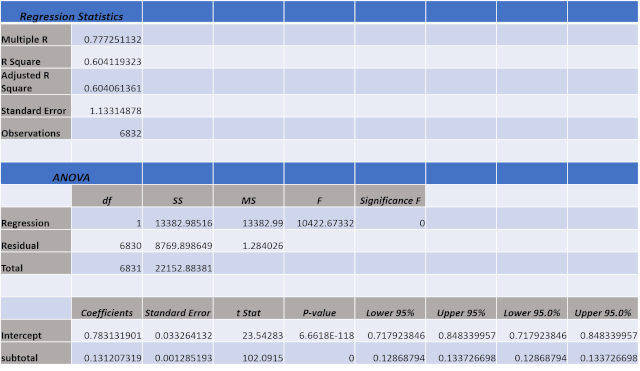
Excel Regression Output
-
Consistency in Results: The Linear Regression outputs obtained from Excel are expected to be consistent with those from Python. The ANOVA table provided by Excel offers a comprehensive overview of the regression analysis, laying the groundwork for further interpretation and analysis.
-
Limitations of Excel: While Excel serves as a convenient tool for basic regression analysis, it falls short in catering to the complexities of Machine Learning. Unlike Python, Excel lacks features such as data splitting and hyperparameter tuning, essential elements for robust Machine Learning models.
Navigating the Analysis
As we progress through this tutorial, we'll dissect and interpret the results obtained from both Excel and Python. By scrutinizing the strengths and limitations of each approach, we'll gain valuable insights into the practical applications of Linear Regression in Artificial Intelligence and Machine Learning. Stay tuned for a comprehensive exploration of regression analysis techniques and their implications for data-driven decision-making.
How to run the Linear Regression with Python Scipy?
Linear Regression analysis using Python's Scipy library offers a robust and efficient approach to extract meaningful insights from datasets. Let's dive into the step-by-step process of performing Linear Regression using Python, leveraging the Scipy library.
1. Set up the Data Frame with Pandas
- Pandas: Utilize the powerful Pandas package to create a structured data frame. Ensure that the CSV file containing the dataset has clear labels for easy organization and readability.
2. Extract Relevant Columns
- Data Extraction: Using Pandas, extract the necessary columns from the dataset. In this example, we focus on the "subtotal" and "tip" columns, which serve as the independent and dependent variables, respectively.
2. Extract Relevant Columns
- Data Extraction: Using Pandas, extract the necessary columns from the dataset. In this example, we focus on the "subtotal" and "tip" columns, which serve as the independent and dependent variables, respectively.
4. Perform Linear Regression
- Regressor Calculation: Utilize the stats.linregress function from Scipy to calculate the slope, intercept, correlation coefficient (r), p-value, and standard error of the regression model.
5. Evaluate Model Performance
- Coefficient of Determination: Assess the model's performance by calculating the coefficient of determination (R-squared) using the r2_score function from the
sklearn.metricsmodule.
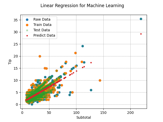
6. Visualize the Results
- Data Visualization: Plot the raw data points, along with the training, testing, and predicted data points, using Matplotlib. This visualization provides a clear understanding of how well the Linear Regression model fits the dataset.
By following these steps, you can effectively run Linear Regression analysis using Python Scipy, enabling you to derive actionable insights and make informed decisions in the realm of Artificial Intelligence and Machine Learning.
import pandas
from scipy import stats

# Load Files & randmoize dataframe
df = pandas.read_csv('tipdata.csv')
df = df.sample(frac=1, random_state=42).reset_index(drop=True)

subtotal = df["subtotal"].values  # Independent Variable DV (X)
tip = df["tip"].values  # Dependent Variable IV (y)

# Split the data into train and test data
from sklearn.model_selection import train_test_split
subtotal_X_train, subtotal_X_test, tip_y_train, tip_y_test = train_test_split(
    subtotal, tip, test_size=0.5, random_state=42)

# The Regressor
slope, intercept, r, p, std_err = stats.linregress(
    subtotal_X_train, tip_y_train)

print("Slope:", round(slope, 3), " |  Intercept:", round(intercept, 2), " |  r:",
      round(r, 3), "|  P value: ", round(p, 5), "|  Std_Error: ", round(std_err, 3))

for tip_pred in tip_y_test:
    tip_pred = slope * subtotal_X_test + intercept

from sklearn.metrics import r2_score
Coef_Det = r2_score(tip_y_test, tip_pred)
print("Coef of Deter R-Squared:", round(Coef_Det, 3))

# Now lets plot the data
import matplotlib.pyplot as plt

plt.scatter(subtotal, tip, label='Raw Data')
plt.scatter(subtotal_X_train, tip_y_train, label='Train Data')
plt.scatter(subtotal_X_test, tip_y_test,
            label='Test Data', marker='*', alpha=0.3)
plt.scatter(subtotal_X_test, tip_pred, label='Predict Data', marker='.')
plt.xlabel("Subtotal")
plt.ylabel("Tip")
plt.title("Linear Regression for Machine Learning  \n")
plt.grid(color='gray', linestyle='--', linewidth=0.5)
plt.legend()
plt.show()
Optimizing Linear Regression with Python SciPy
In our quest for efficient Linear Regression analysis, we turn to the linregress function from the Python SciPy statistical package. Leveraging this powerful tool, we can streamline our analysis process and achieve robust results that stand the test of comparison against other widely used packages like Excel, R, or Java.
slope, intercept, r, p, std_err = stats.linregress(subtotal,tip)
Exploring the Output
The linregress function furnishes us with a comprehensive output, including the slope, intercept, Pearson coefficient (r), p-value, and standard error derived from the training data subsets. In our case, the dependent variable is the tip, while the independent variable is the subtotal.
It is easy to verify that the output of the linregress compares very well with the results shown in the Excel ANOVA table. Note, however, that the Excel output is for the whole data set of all the points while the linregress includes only half of the data for training the algorithm the other 50% is for testing the algorithm.
Slope: 0.13  |  Intercept: 0.83  |  r: 0.763 |  P value:  0.0 |  Std_Error:  0.002
Coef of Deter R-Squared: 0.623
Understanding Coefficient of Determination (R-Squared)
The coefficient of determination, often denoted as R-squared or R2, plays a pivotal role in assessing the predictive power of our model. When r is squared, we obtain the R-squared value, representing the proportion of the variance in the dependent variable that is predictable from the independent variable.
- First Coefficient of Determination (from the linregress train data): r to the power of 2 (0.763)2 = 0.582
- Second Coefficient of Determination (from the sklearn python library comparing the test data with the predicted values i.e. the tip_test data set vs tip_pred test data): 0.62
Both coefficients align closely with the Excel output of 0.604, showcasing the consistency and reliability of our analysis across different platforms.
Ensuring Clarity in Notation
To avoid confusion, it's imperative to maintain clarity in our notation. We distinguish between the Pearson Correlation Coefficient (r) and the Coefficient of Determination (R2) R-Square, or simply R2, ensuring precision in our analysis.
If we change the size of the train vs test subsets we will get slightly different results.
Examining the Scatter Plot
A visual inspection of the scatter plot reveals the presence of numerous outliers within our dataset, a phenomenon that warrants further discussion and analysis in subsequent stages of our exploration.
By harnessing the capabilities of Python SciPy and adopting a meticulous approach to our analysis, we equip ourselves with the tools necessary to conduct Linear Regression with confidence and precision in the realm of Machine Learning and Artificial Intelligence.
How to perform Linear Regression with OLS Statsmodel?
When it comes to Linear Regression analysis, leveraging the OLS (Ordinary Least Squares) library from Statsmodel is akin to wielding a precision tool in the realm of data science. Comparable to its counterpart, linregress, OLS offers a seamless pathway to unlocking insights from your dataset with unparalleled accuracy and efficiency.
Advantages of OLS Statsmodel
One of the standout features of OLS is its comprehensive summary report, a treasure trove of invaluable insights that provides a deeper understanding of your regression model. From coefficients to confidence levels, this built-in report is as close as it gets to Excel empowers analysts to glean actionable insights and make informed decisions with confidence.
Lets jump in the OLS regressor python code:
import pandas

# Load Files
df = pandas.read_csv('tipdata.csv')
df = df.sample(frac=1, random_state=42).reset_index(drop=True)

subtotal = df["subtotal"].values
tip = df["tip"].values

# Split the data into train and test data
from sklearn.model_selection import train_test_split
subtotal_X_train, subtotal_X_test, tip_y_train, tip_y_test = train_test_split(
    subtotal, tip, test_size=0.5, random_state=42)


import statsmodels.api as sm
# Do not forget to add the constant most of us do!
subtotal_X_train = sm.add_constant(subtotal_X_train)
model = sm.OLS(tip_y_train, subtotal_X_train).fit()
print(model.summary())

# Prediction method 1 with for loop
slope = model.params[1]
intercept = model.params[0]

for tip_pred_M1 in tip_y_test:
    tip_pred_M1 = slope * subtotal_X_test + intercept

from sklearn.metrics import r2_score
Coef_Det = r2_score(tip_y_test, tip_pred_M1)
print("Coef of Deter R-Squared Mthd_1:", round(Coef_Det, 3))


# Prediction method 2 with statsmodel predict fuction
subtotal_X_test = sm.add_constant(subtotal_X_test)
tip_pred = model.predict(subtotal_X_test)

Coef_Det = r2_score(tip_y_test, tip_pred)
print("Coef of Deter R-Squared Mthd_2:", round(Coef_Det, 3))
Interpreting Results
The summary report of the OLS model is displayed next, offering a comprehensive view of key parameters such as the slope, intercept, and coefficient. As demonstrated in the code, these crucial metrics can be effortlessly extracted programmatically, enabling analysts to delve deeper into the intricacies of their regression model.
Within the code snippet provided, we meticulously partitioned the data into training and test subsets, a fundamental step in ensuring the robustness and reliability of our analysis. Employing two distinct methods for predicting Y as a function of X—specifically, predicting the tip based on the subtotal—revealed a noteworthy consistency: both the custom loop function and built-in prediction methods yielded identical Coefficient of Determination values. This harmonious outcome underscores the precision and accuracy of the OLS regression model, reaffirming its efficacy as a cornerstone tool in the realm of data science.
.
                            OLS Regression Results
==============================================================================
Dep. Variable:                      y   R-squared:                       0.581
Model:                            OLS   Adj. R-squared:                  0.581
Method:                 Least Squares   F-statistic:                     4742.
Date:                Sun, 27 Feb 2021   Prob (F-statistic):               0.00
Time:                        00:59:50   Log-Likelihood:                -5227.2
No. Observations:                3416   AIC:                         1.046e+04
Df Residuals:                    3414   BIC:                         1.047e+04
Df Model:                           1
Covariance Type:            nonrobust
==============================================================================
                 coef    std err          t      P>|t|      [0.025      0.975]
------------------------------------------------------------------------------
const          0.8273      0.048     17.301      0.000       0.734       0.921
x1             0.1297      0.002     68.864      0.000       0.126       0.133
==============================================================================
Omnibus:                     1160.361   Durbin-Watson:                   1.970
Prob(Omnibus):                  0.000   Jarque-Bera (JB):            35288.718
Skew:                           0.989   Prob(JB):                         0.00
Kurtosis:                      18.621   Cond. No.                         63.5
==============================================================================

Notes:
[1] Standard Errors assume that the covariance matrix of the errors is correctly specified.

Coef of Deter R-Squared Mthd_1: 0.623
Coef of Deter R-Squared Mthd_2: 0.623
How to use Linear Regression with Python Sklearn?
Similarly, we wrote a quick code to model the dataset with the Sklearn LinearRegression package.
import pandas
from sklearn.linear_model import LinearRegression

# Load Files
df = pandas.read_csv('tipdata.csv')
df = df.sample(frac=1, random_state=42).reset_index(drop=True)

subtotal = df["subtotal"].values
tip = df["tip"].values

#Use Reshape otherwise headache errors
subtotal = subtotal.reshape(-1, 1)

# Split the data into train and test data
from sklearn.model_selection import train_test_split
subtotal_X_train, subtotal_X_test, tip_y_train, tip_y_test = train_test_split(
    subtotal, tip, test_size=0.5, random_state=42)

model = LinearRegression().fit(subtotal_X_train, tip_y_train)
tip_pred = model.predict(subtotal_X_test)

from sklearn.metrics import r2_score
Coef_Det = r2_score(tip_y_test, tip_pred)  # compare y test to y predict

print("Slope: ", round(model.coef_[0], 3))
print("Intercept: ", round(model.intercept_, 3))
print("Coef of Deter R-Squared: ", round(Coef_Det, 3))
The results from the Sklearn regressor are shown next. Sklearn does not provide a summary report like the OLS method, however, the coefficients could be either printed or data scientists could write their class functions. One quick comment is that the results of Sklearn compare very well with the other regressors we discussed in this article.
Slope:  0.13
Intercept:  0.827
Coef of Deter R-Squared:  0.623
Comparing Methods and Performance
So far we described 4 methods to run linear regression Excel, Scipy, OLS, and Sklearn. The advantage of one method over the others is subjective. In production, real life, depending on the situation machine learning experts need to run and compare all these methods, and based on needs (performance vs speed) someone could determine the best solution to solve their specific problem.
- For web applications, if Linear Regression is required for predictions, it might not be easily possible to use Excel. On the other hand, someone could easily call and run Python libraries.
- From the 3 Python Scipy, OLS, and Sklearn, it seemed that Sklearn compiled the regression much faster than the other libraries. Speed becomes more important as the dataset grows larger. During our trial runs, we used Eclipse with CPython however if speed is critical someone could use the PyPy it is estimated that PyPy is approximately 94 times faster, running similar code in just 0.22 seconds as opposed to 20 seconds. Again that is under specific large datasets conditions.
Understand Linear Regression Models
Linear Regression is a method that provides us with a linear model Y = β0+β1X+ε
Rearranged into Y = β1X+β0+ε
For the time being, we will ignore ε but must keep in mind that ε is of critical importance and it is called the error or residual!
Rewritten as Y = β1X+β0, this is nothing more than a linear function that was taught in 8th grade.
β1 is called the Slope
β0 is the Intercept
After substitution from the result and rewrite Y = (0.13)*X+$0.83 or $tip = 0.13($subtotal) + $0.83
So for each additional dollar in the ticket (subtotal), we expect a tip increase of 13 cents. Now, how about that $0.83? Many do not know how to describe the β0, that is why it is critical to understand the physical problem being solved. In this specific case, β0 is the opportunity loss with each delivery or lack of. Meaning instead of making the full amount which is the subtotal of the bill x 0.13 + $0.83, the driver is just making an average of $0.83 by sitting down and doing nothing. Also, note that with other datasets, the intercept β0 could be negative at which point the opportunity loss is clearer.
So to predict the tip associated with a subtotal of $25, we just substitute: $tip = (0.13)*$25+$0.83 = $3.25+ $0.83 = $4.08.
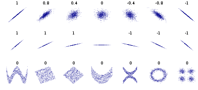
Understand Pearson Coefficient known as Correlation Coefficient
In our model, the Pearson Correlation Coefficient is 0.763. The Pearson Coefficient tells us how LINEAR is the co-relationship between a bivariate (X,Y), and is NOT how well the model fits the observation. Pearson Correlation Coefficient could be any number between 1 and -1.
- A Pearson Correlation Coefficient of zero means that there is no LINEAR relationship between the set.
- An ideal Pearson Correlation Coefficient of 1 or -1 means all the data in Y could be explained by a linear equation having a slope and an intercept where the error is zero.
So at 0.763 Pearson r, we could conclude that there is a good Linearity between our BiVariate, subtotal, and tip.
There are other correlation coefficients that we encourage you to read about from a textbook and understand. But in particular, is to practice and apply those correlations to real-life problems.
Assessing the Linear Regression model: Unveiling Performance Metrics?
In the realm of Data Science, the term "Good" is not absolute but comparative. A Good Model stands out by delivering superior performance when juxtaposed with its counterparts. To gauge performance effectively, a standardized metric becomes indispensable. Herein lies the significance of the Coefficient of Determination, commonly denoted as R-squared (R2).
Explanation of R square, Coefficient of Determination
R-squared, or the Coefficient of Determination, epitomizes the goodness of fit in statistical modeling. It elucidates the extent to which the variation in the Dependent Variable is elucidated by the Independent Variable. Linear Regression, being an optimization algorithm, endeavors to minimize R2.
In our scenario, R2 hovers around 60.04%, implying that 60.04% of the variance in Y (the tip amount) finds explanation in X (the subtotal of the delivery order). However, a pertinent question arises: What about the remaining 39.96%? Enter ε, the residual error term.
In Linear Regression, the Coefficient of Determination is computed as the square of the Pearson Correlation Coefficient. A complementary method yielding identical results is the ratio of the Sum Square of the Residual (SSR) to the Sum Square of the Total Error (SST). For instance, referencing the Excel output provided earlier, R2 is calculated as SSR/SST, where R2 = Regression / Total = 13382/22152 = 0.604119.
While this article delves into the fundamentals, advanced practitioners are encouraged to delve deeper into concepts such as SSR, SST, and SSE for a comprehensive understanding of model evaluation.